Visualizing the bivariate normal distribution and its properties

The normal distribution plays a central role in statistics and natural sciences. There are multiple natural phenomena (e.g. population height) that are closely described by a normal distribution. The picture that comes to mind when talking about the normal distribution is that of a bell shaped curved. Once we consider higher dimension random variables it s more difficult, or even impossible, drawing pictures to help us grasp the variables’ distribution features.

Personally, I consider myself a visual learner. Having a mental picture of something helps me pin down the concepts better, even when plotting is not an option. That is why I thought it would be interesting visualizing the bivariate normal distribution and its properties.

I have plotted here two bivariate normal distributions. To keep things simple, both random variables of the bivariate normal have mean 0 and a standard deviation of 1. I concentrate on two cases: positive and null correlation.

Suppose that you are studying the market of magazines and newspapers. You know that money people spend in both items is distributed according to a bivariate normal ¹. Let’s use $M$ for money spent in magazines, and $N$ for money spent in Newspapers.

Setting 1 - no covariance

In setting 1 we assume that there is no correlation between money spent in both items. In other words, observing the spending patterns in magazines does not convey information about how much money will be spent in newspapers. If that is so, here is how its bivariate distribution looks like:

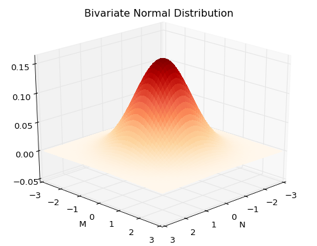
While usually when it comes to distributions, zero correlation does not mean independence, this is not the case for the bivariate distribution. It is enough to know that there is no correlation between the random variables, to claim they are independent.

The most intuitive way to understand independence, is to answer the question: does the value certain variable takes, informs me about the value the other variable would take? Going back to the example, one could ask the following question: what is the probability that a customer will spend from 1 to 1.5 dollars in newspapers given that he spent one dollar in magazines. Let’s see how is possible to see the variables’ independence in the graph.

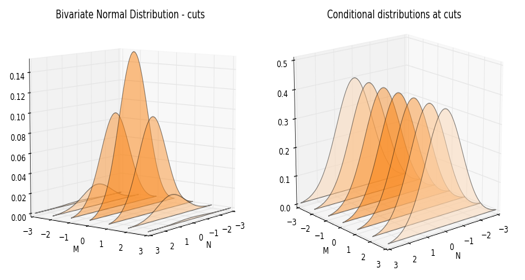
In the graphs above, first we observe the bivariate distribution at different cuts. These cuts are taken at specific values of the variable money spent in magazines, $M$. Next to it, is a graph of the conditional distributions at those values. The conditional distribution is the same as the joint observed in the right, with the difference that the density is normalilzed so its total probability sums up to one.

The independence of these random variables can be grasped by the fact that the distribution of $N$ does not move. It basically remains unaffected, no matter what value $M$ takes. In other words, knowing how much someone spends in magazines, does not help us determine how much she will spend in newspapers. This is easily observed by the fact that the conditional distributions of $N$ at different values of $M$ are a mirror of each other.

As we are talking about conditioning, another interesting property of bivariate random normals is related to the conditional expectation: The conditional expectation of a random variable is a linear function of the other. How would this play out in a world with zero correlation?

If what I have said is correct, then the conditional expectation of money spent in newspaper should not depend on values taken $M$. Here is a way to observe this property. Using the same cuts as before, I plot a scatter plot to observe the conditional distribution in the $M$ and $N$ dimension.

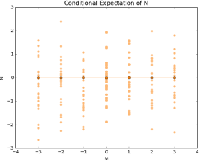
The horizontal line is proof of that independence. Basically, the expectations remain unmoved, no matter what values the other variable takes. Knowing how much money clients spend on magazines, does not tell us anything about their purchase patterns of newspapers.

Setting 2 - with correlation

Let’s keep our previous example. The only difference now, is that these variables are highly and positively correlated (0.8). People that buy lots of magazines, also buy lots of newspapers. This is how the bivariate distribution picture looks like.

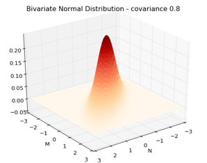
Note how the picture varies from the case without correlation. Before we had a perfect mountain. No matter the position from where we looked, the distribution always looked the same from base to top. Here things are different. We can see that the distribution concentrates exactly in those places where both variables show similar values. This makes sense. Positive correlation entails that low values spent on magazines are also related to low spending in newspapers. Of course, high values of spending in one are also related to high values of the other random variable.

Now look how the “distributional cuts” and conditional distributions look like. To help the comparison, the cuts and conditioning are at the same values of the variable $M$ as before.

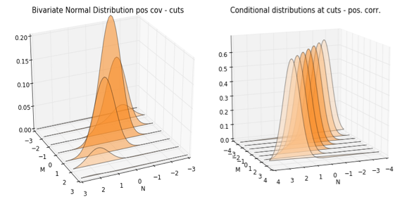
The most striking difference between the previous setting is the movement of each distribution at each of the cuts. These shifts are more obvious when we compare conditional distributions. In the zero correlation world, the distributions were pretty much a mirror of each other. In this case of strong correlation, one can observe how these distribution, belonging each to a particular realized value of $M$, are shifted or displaced. In particular, the higher values this variable takes, the more the distribution shifts to higher values, too. Unsurprisingly, this again is a consequence of the positive correlation between both random variables.

Now let’s look at how the conditional expectation looks in this case. As mentioned before, bivariate normal random variables have a linear conditional expectation. This can be seen in the following picture:

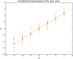
We can clearly see how the expectation is connected by an upward sloping line. In this case, knowing how much money a client spends in one product, gives you valuable information to infer how much on average she will spend on the other.

Hope this pictures give you a clear idea about the bivariate normal distribution. You can always check the code and continue playing with the graphs and assumptions in the related notebook.